Micro Servo Data Collection, Parameter Identification, and Modeling: Parts 1-4
Introduction
Finding good information on low-cost servos is difficult. In the next articles, I will describe my informal journey finding and identifying the motor parameters for a SG90 9-gram servo motor. These motors are ubiquitous at the low end of robotics parts, and are thus quite attractive for making affordable robots in the classroom. The quality of these motors varies widely, however, and little information has been collected on them in one place. Different manufacturers often give only some specifications.
So here is my attempt at modeling an SG90 servo using as much information as I could find on the web, plus a little elbow grease to put it all together.
Parts
I used only tools I would imagine a resourceful citizen scientist would have, including:
- A cell phone for capturing video
- A selfie-stick tripod and mount for attaching my cell phone (you can use a chair, books, tape, etc to rig up your own mount if you don’t have one.)
- A single SG-90 servo.
- A single AA battery for some added inertia
- Wire to physically attach the battery
- A breadboard
- An ESP32 for sending position commands
Other tools that would have greatly helped include a multimeter with current sensing and USB data output, oscilloscope, or current sensor. These tools would have let me measure current usage over time, including at startup/stall and in no-load conditions. Without this tool, I had to rely on manufacturers’ data sheets and my own memory of prior tests.
Software
I already have my computer set up with the following tools
- VSCode for interacting with the ESP32 and micropython
- An ESP32 flashed with micropython
- An anaconda distribution with mujoco and jupyter lab installed
Procedure
Note: In case you don’t have the parts on hand you can still follow along with the data. The tracker project file (with video) is linked here and the .csv output can be found here
Part 1: The Experiment
I flashed micropython onto the ESP32 and crafted a simple program to alternate the servo 180 degrees every 2 seconds. I won’t go into detail on this step here, but feel free to poke around my website for other resources on ESP32, micropython, and servos. The code looked like this:
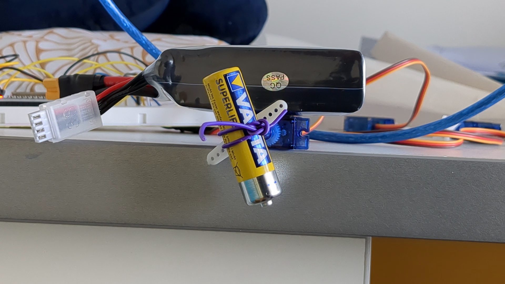
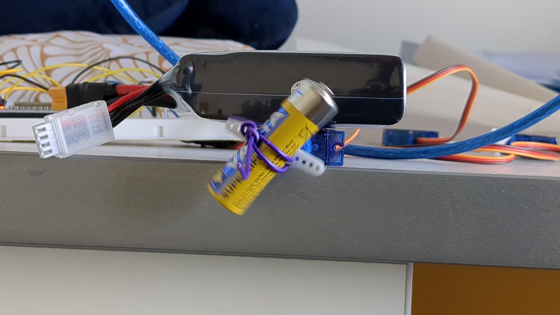
from machine import Pin, PWM
from time import sleep
frequency = 50
range_low = 28
range_high = 122

servo1 = PWM(Pin(14),frequency)

while(True):
    servo1.duty(range_low)
    sleep(1)
    servo1.duty(range_high)
    sleep(1)
I then plugged in my ESP32 to a half-size breadboard and wired up my servo. I hung the end of the servo off the edge of a desk and weighted it down so it wouldn’t move.
I wrapped a wire around my AA battery to rigidly attach it to the servo’s horn. I mounted the battery so it was mounted symmetrically about the rotational center of the servo.
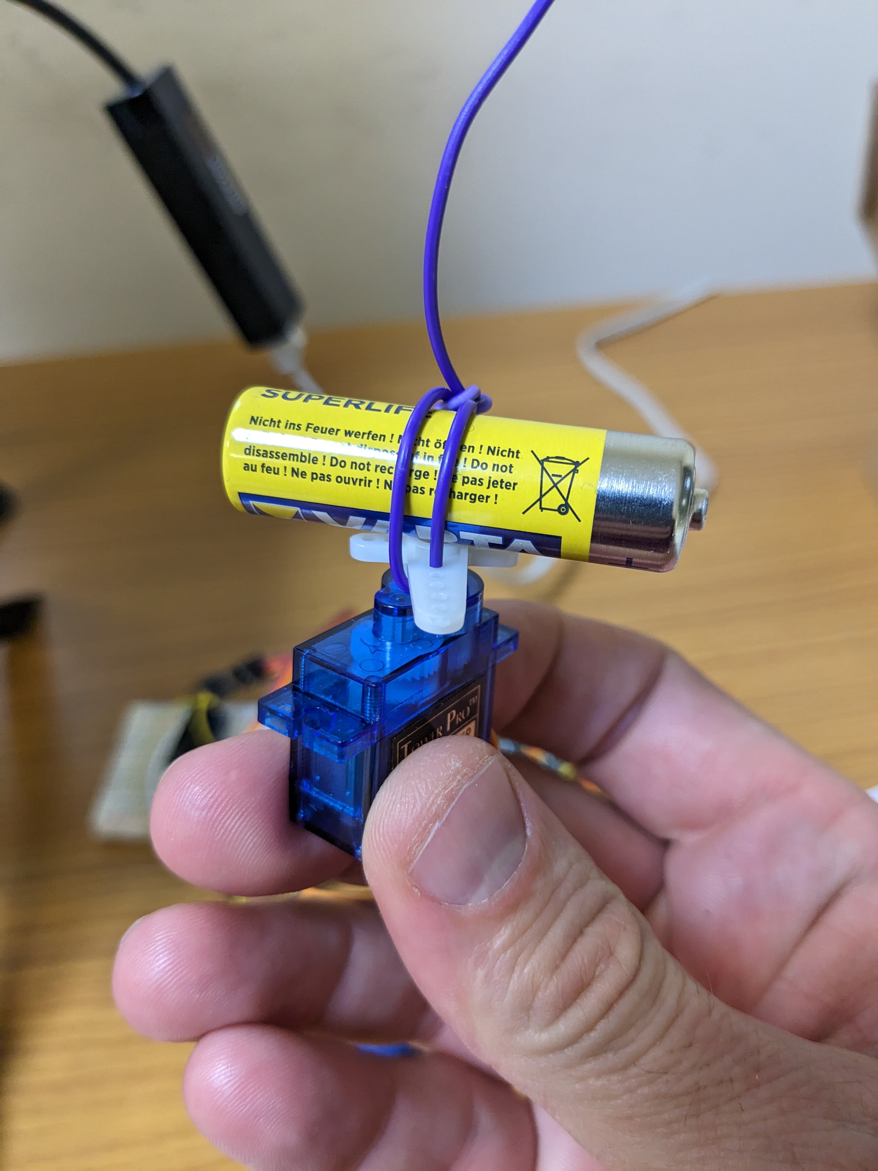
My Inertial Load
I weighed my battery for use later
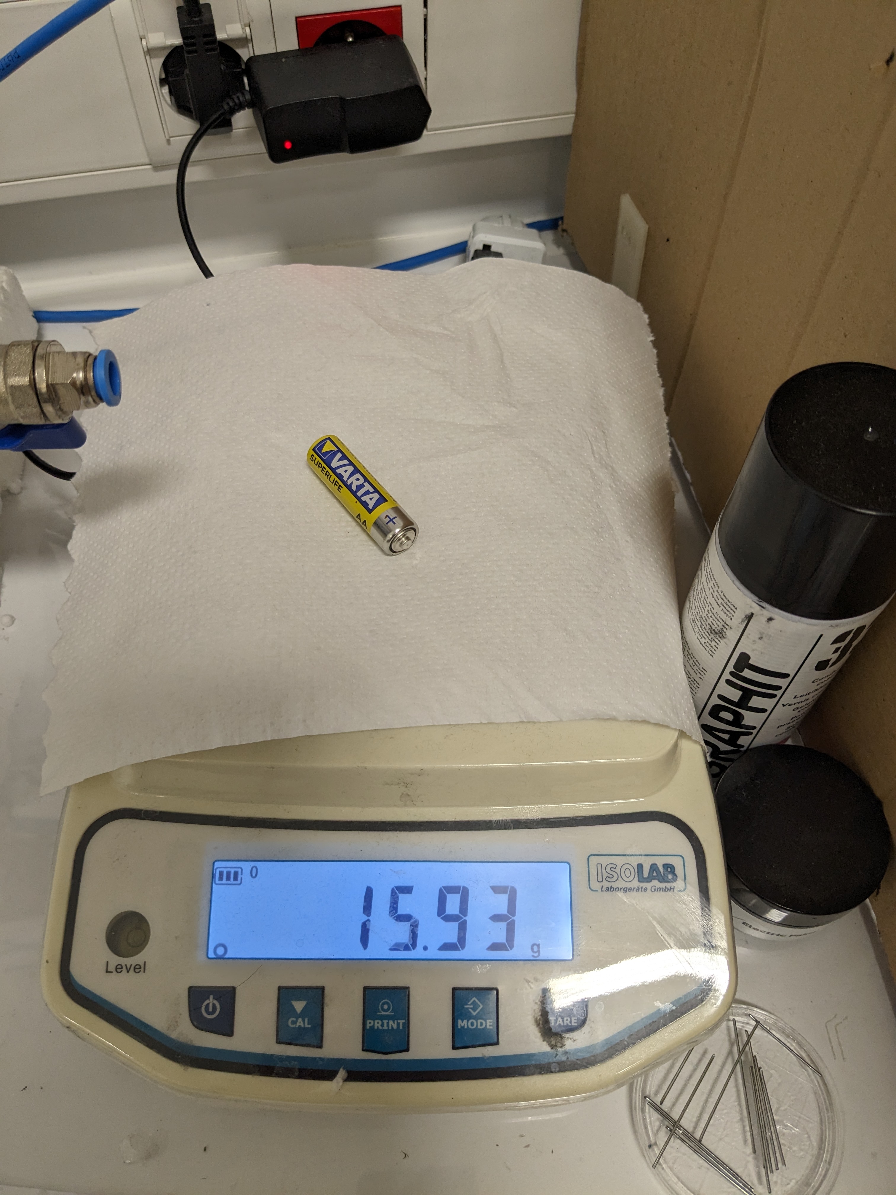
Weighing my mass
I used a small tripod to hold my cell phone approximately 12 inches away from my scene. I made sure my servo was in the center of my frame, that my camera was perpendicular to the plane of my experiment, and that my zoom was such that I was not using the “fish-eye” lens of my camera…in the case of a google pixel 6a, anything less than 1x uses the fish-eye lens that exhibits more warping around the edges. I did not bother to zoom in much, though, since I am not sure where digital zoom takes over. (Digital zoom doesn’t add any more information to the experiment, and can result in a worse image due to the extra image processing performed by the camera.)
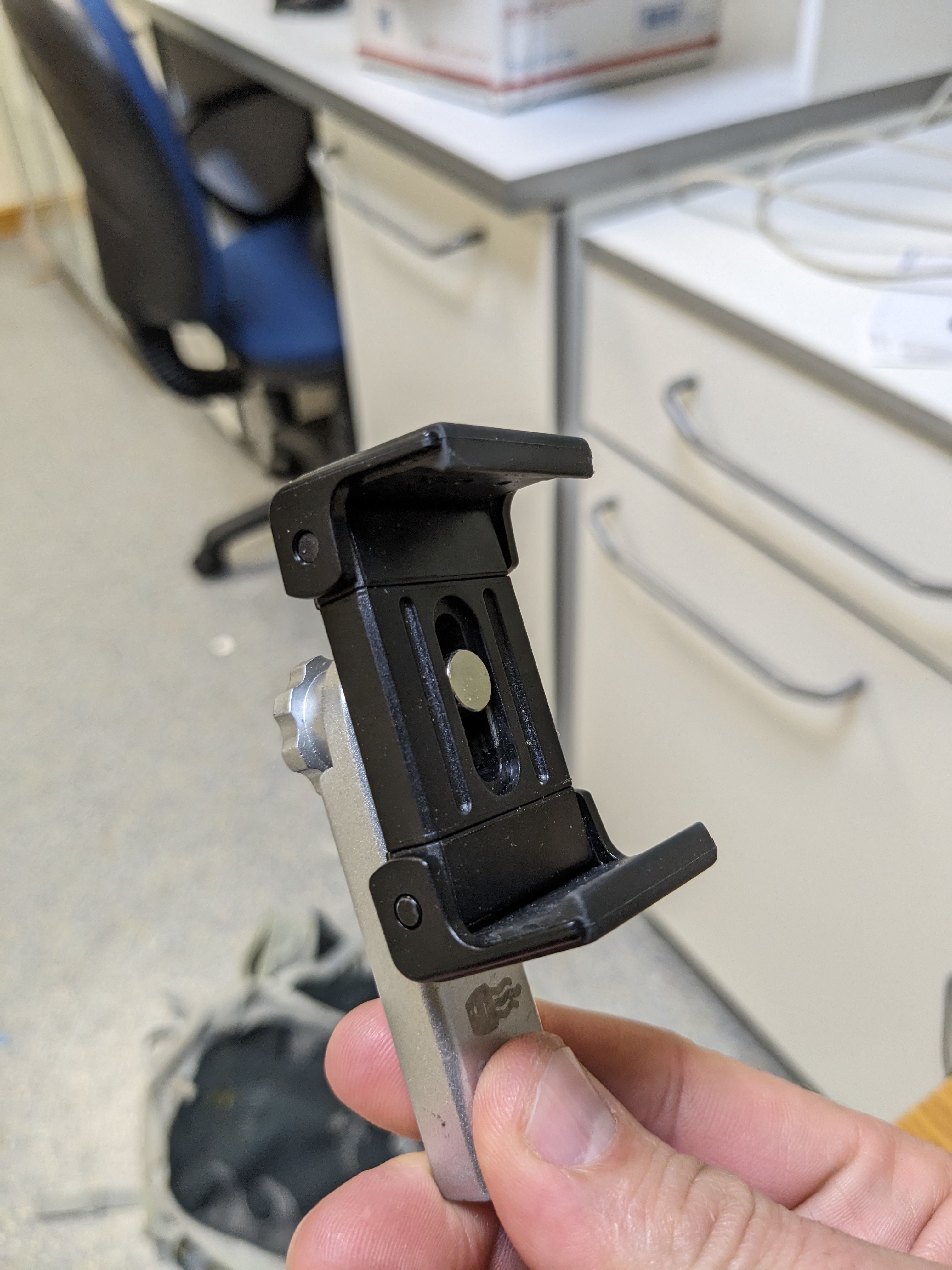
The camera mount
Note 1: It is important that your scene is as centered as possible in your image, and that the plane of motion is as perpendicular as possible to your camera lens’s radial axis. This will minimize the amount of warping seen in your image.
Note 2: It should be noted that this is an informal approach to optical tracking. Camera calibration and knowledge of how lens distortion works should be utilized at this step when adapting my approach to a lab setting, but again, this article is focused on “good-enough” citizen science techniques, or techniques you can actually apply in a single, 75-minute class.
I took several practice videos and checked them to ensure the camera didn’t move, the base of the servo didn’t shake or move, and that my scene was well-lit and in focus.
The servo stopped; no blur visible
The servo moving; it is still relatively easy to identify key points
Part 2: Image tracking
Tracker Screenshot
I installed tracker on a Windows computer and imported my video. I identified several high-contrast points that remained visible even during the blurry bits when the servo was rotating. Tracker has the ability to follow marked points forward in time once you mark them. It follows the key point for as many frames as it can. I would call this a semi-automatic process. In my case, I found tracker’s tools to be only moderately helpful as the quality of my video was so low. But I was able to manually find most points tracker couldn’t; tracker filled in the gaps when the servo was not moving.
I have a full tutorial on tracker associated with my foldable robotics class. Please see that for more information (as well as more tips on scene setup). A couple tips here though:
- I used the edge of the desk as my x-axis reference line, to ensure the x-y coordinate system matched up with a planar model with gravity in the -y direction.
I output the data as a .csv file. Opening the file, I removed the two excess lines above the column labels. the Pandas package in python expects only one row above data, for heading labels. Once done, I saved the file to the same file name.
Part 3: Massaging the Data
In this part, lets summarize the information we have and the information we need. First, we have a given orientation of our recorded image frames because we captured the (supposedly) horizontal level of the desk. It would have been better to verify the level of the desk…but it is what it is. We have two tracked points. We don’t have the location of the servo relative to those points, and we don’t specifically have the center of rotation. That will be the first issue. We also don’t exactly know the mass distribution of the battery as it was actually attached to the servo, but for this experiment we will assume we did a good job at centering it. A potential improvement on the last step would be to measure the distance to the battery’s boundaries at specific points in time to confirm it was roughly centered around the servo’s rotational axis. We can go back and add that later to the tracker project if we feel we need more precision.
Now let’s talk about what we need. Do we need the position of the servo? no. Do we need the position of particular points of the battery? No.
All we really want to know is how fast does the servo accelerate with an extra inertia attached to its output.
All other data can be obtained through electrical experiments, off the manufacturer’s data sheet, or through first principles equations. So let’s work on converting our captured data points into an angular measurement, $\theta$, that we can then compare to a dynamic model.
First, let’s import some necessary packages in python…
import pandas
import scipy.signal as ss
import scipy.optimize as so
import numpy
import matplotlib.pyplot as plt
import math
Next, we import data collected by tracker and identify the useful columns
Reminder: You will need to open the .csv file to remove the first two rows. Pandas expects just one row for column names above the data
data = pandas.read_csv('data.csv')
data.columns
Index(['t', 'x', 'y', 'x.1', 'y.1'], dtype='object')
Extract the time and position data of our markers
t = data['t']
Challenge: Finding the center of rotation
The issue with my simple experiment was that it was quite hard to mark or estimate the center of rotation prior to the experiment. Now that I have video data, though, I can make an estimate abou the center of rotation by using the tracking data obtained from my marked points. In the next few chunks of code you’ll see how I went about identifying the best guess for the center of rotation.
First, make a guess for the center of rotation by finding the mean of all the x and y data of our first point. This is rough but it should be close enough for an optimizer to do the rest
xini = data['x'].mean()
yini = data['y'].mean()
ini = numpy.array([xini,yini])
print(ini)
[2.55072079 0.21735663]
Next, create a function that finds the sum of squared radii given an x,y coordinate guess for the center of rotation, across the two points tracked. By obtaining the distance from the guessed center to each point over all the data, the true center should minimize the sum of all distances to all tracked points.
def fun(guess):
    # break out guess into two variables, x0 and y0
    x0,y0 = guess
    # start with zero error
    error = 0
    # sum the squared length to point 1 over all time and add to error
    error += ((data['x']-x0)**2+(data['y']-y0)**2).sum()
    # sum the squared length to point 2 over all time and add to error
    error += ((data['x.1']-x0)**2+(data['y.1']-y0)**2).sum()
    # take the square root
    error = error**.5
    # return the error
    return error
The function, evaluated at the initial guess should provide a baseline error that can go lower still
print(fun(ini))
18.010570547148244
Run the minimization and check the result
result = so.minimize(fun,ini)
result
  message: Optimization terminated successfully.
  success: True
   status: 0
      fun: 17.655446173747816
        x: [ 2.719e+00  2.522e-01]
      nit: 4
      jac: [-7.153e-07  0.000e+00]
 hess_inv: [[ 8.129e-02 -1.918e-01]
            [-1.918e-01  9.600e-01]]
     nfev: 21
     njev: 7
Compute the vectors from the origin to the two tracked points. This will effectively shift the original tracked points to move about the result of our optimization, the selected center of rotation in the video.
v1 = numpy.array([data['x']-result.x[0],(data['y']-result.x[1])]).T
v2 = numpy.array([data['x.1']-result.x[0],(data['y.1']-result.x[1])]).T
Plot the vectors over time, along with a dot at the origin.
plt.plot(v1[:,0],v1[:,1])
plt.plot(v2[:,0],v2[:,1])
plt.plot(0,0,'ro')
plt.axis('equal')
(-1.0102513998296843,
 0.8169597001703157,
 -1.101215392464636,
 1.0497984175353638)
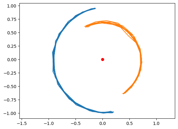
Circular Motion
The angle of each vector can be computed by taking the arctan of the x and y components of vector 1 and 2. Plot the result.
theta_v1 = numpy.arctan2(v1[:,1],v1[:,0])
theta_v2 = numpy.arctan2(v2[:,1],v2[:,0])
plt.plot(t,theta_v1)
plt.plot(t,theta_v2)
[<matplotlib.lines.Line2D at 0x7f4e40ade990>]
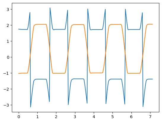
Rotation Angle with atan2 jumps.
This data has some discrete jumps in it, though. Why? The issue is that the theta value recovered “jumps” when it exceeds $|\pi|$. We can further work with the data to “unwrap this value. Any value that jumps more than $\pi$ between individual timesteps by the arctan2 function can be interpreted to actually be continuously increasing (or decreasing) past that value. We just need to keep track of how many times from the beginning of our data we have crossed this threshold, and add it to our original measurement. Thus, we have the unwrap() function.
Note: Scipy / Numpy has an unwrap function but it doesn’t seem to work for me…thus, I wrote my own.
def unwrap(theta,period):
    #create a holder for our new theta measurement, theta2, and seed it with the initial value of theta.
    theta2 = [theta[0]]
    #we need to compare our current theta measurement against the previous one.  thus, we store the initial value so there are no initial jumps.
    last_theta = theta[0]
    #create a holder for the number of times we have transitioned through another period
    mem = 0

    # Starting at our 2nd data point(index 1)
    for t_ii,item in zip(t[1:],theta[1:]):
        #compare our current theta against the last theta
        dt = (item - last_theta)
        #check if there is a big jump in the positive or negative direction, and if there is, subtract or add one period value to mem
        if dt>(period/2):
            mem-=period
        if dt<(-period/2):
            mem+=period

        # compute the corrected value of theta and add to theta2
        theta2.append(item+mem)
        # update last_theta
        last_theta = item

    # reform theta2 as a numpy array
    theta2 = numpy.array(theta2)
    # and return it
    return theta2
now run the function on our two guesses for vector 1 and vector 2
theta_v1_u = unwrap(theta_v1,2*math.pi)
theta_v2_u = unwrap(theta_v2,2*math.pi)
By subtracting the initial values for theta_1 and theta_2 we obtain two guesses for the same angle value.
theta_v1_u-=theta_v1_u.min()
theta_v2_u-=theta_v2_u.min()
Plot the corrected values
plt.plot(t,theta_v1_u)
plt.plot(t,theta_v2_u)
[<matplotlib.lines.Line2D at 0x7f4e4150a010>]
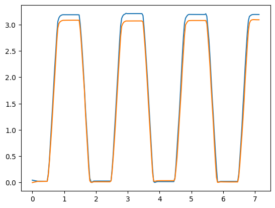
The two measurements
Compute the average of these two samples. Adding even more points to this analysis would give us a more accurate measurement of theta.
theta_u = (theta_v1_u+theta_v2_u)/2
plt.plot(t,theta_v1_u,'b:')
plt.plot(t,theta_v2_u,'b:')
plt.plot(t,theta_u,'r-')
[<matplotlib.lines.Line2D at 0x7f4e40b67e50>]
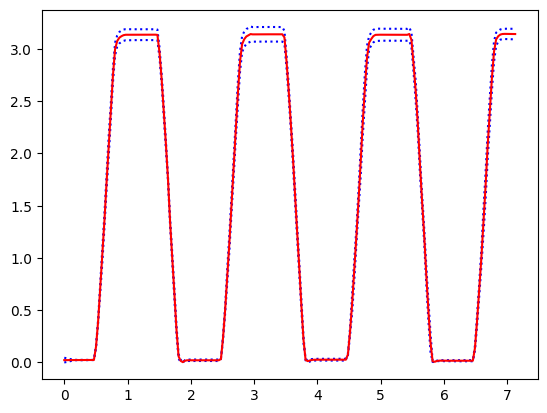
Average of the two measurements
Out of curiosity, what is the maximum value of our guessed value of theta?
theta_u.max()*180/math.pi
180.13261077941166
Wow!
Part 4: Guessing the input signal
Because of the informal nature of the experiment, it is hard to capture the actual PWM signal and compare against the output motion of our servo. To make a good guess, however, we can reconstruct the step signal sent by the ESP32 and place it one time-step in front of any observed motion in the frames.
First, we make a filter to only look at data values less than a second, just to zoom in on the first transition
time_filter = t<1
We then find the index of the first point in time where theta starts moving in order to guess the time-delay of our first command signal. We find it hueristically by finding the theta value that more than 1% of the full range of observed thetas from min(theta), starting at t=0. We save that index as jj, and identify the starting time, t_0, using the index
jj = theta_u[time_filter] > (theta_u[time_filter].max()
                             - theta_u[time_filter].min())*.01
    + theta_u[time_filter].min()

t_0_kk = (t[time_filter][jj]).idxmin()
t_0 = t[t_0_kk]
t_0
0.5015946
We then plot the moment motion starts on top of the adjusted theta values:
plt.plot(t[time_filter],theta_u[time_filter])
plt.plot(t[t_0_kk],theta_u[t_0_kk],'ro')
[<matplotlib.lines.Line2D at 0x7f4e4153e910>]
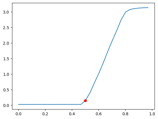
The point motion starts
This means the signal must have been sent at least one time-step before this. Maybe more, but the best-case scenario for lag would be one frame of video.
Lets create a function that can generate a step function with the following parameters
A: amplitudef: frequencyw: width (as a fraction of the full time step) of the positive portion of the square waveb: y-offset
A = math.pi
f = .5
w = .5
b = 0

def square(t,A,f,w,b,t_0):
    y = (t-t_0)*f
    y = y%1
    y = (y<w)*1
    y = A*y +b
    return y
y = square(t,A,f,w,b,t_0)
plt.plot(t[time_filter],theta_u[time_filter])
plt.plot(t[time_filter],y[time_filter])
plt.plot(t[t_0_kk],theta_u[t_0_kk],'ro')
[<matplotlib.lines.Line2D at 0x7f4e40c70fd0>]
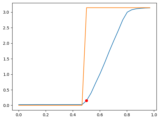
The guessed control signal
Now lets check our results over all the collected data
plt.plot(t,y)
plt.plot(t,theta_u)
[<matplotlib.lines.Line2D at 0x7f4e40c74850>]
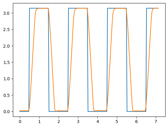
Checking our work
it looks good! Now let’s save some of our work for use in other code
data = {}
data['A'] = A
data['f'] = f
data['b'] = b
data['w'] = w
data['t'] = t
data['t_0'] = t_0
data['theta_u'] = theta_u
import yaml
with open('servo_data_collection.yml','w') as f:
    yaml.dump(data,f)
The resulting .yaml file can be found here
In the next writeup, I will continue, showing off how I modeled the motor and controller, and then obtained some best-fit model parameters.