Micro Servo Data Collection, Parameter Identification, and Modeling: Parts 5 and 6
Introduction
In the last article I took some data from a small, off-the-shelf servo, the SG90, 9 gram micro-servo. In this article, I continue with modeling and parameter fitting. This work was done to prepare for the class I developed, called Flexible Robotics. This is an undergraduate course with a focus on mechanism design and kinematics, experimentation, prototyping, parameter ID and design optimization. I introduced the python interface to MuJoCo as our tool of choice for modeling and simulation in the second half of the course, as it is both relativly easy to pick up and it motivates many interesting discussions about contact, compliance, and modeling decisions. So this article focuses on how to model the servo using MuJoCo.
Steps
Part 5: MuJoCo-based model
This step involves developing a MuJoCo model matching the experimental setup, and using it in conjunction with the collected data in identifying the remaining unknown parameters.
First we import required packages and modules
import matplotlib.pyplot as plt
import numpy
import math
import yaml
import mujoco
import numpy
import mediapy as media
Since this is a separate ipython notebook, I am repeating some of my previous work (shame!). I define a square-wave function for emulating the control signal sent to the pwm model.
def square(t,A,f,w,b,t_0):
    y = (t-t_0)*f
    y = y%1
    y = (y<w)*1
    y = A*y +b
    return y
Motor Modeling
This is where there is some guesswork involved. I pored over a number of datasheets (linked below) to identify common parameters across many different manufacturers. I know that the SG90 may not share the same innards across manufacturers, and in the past I’ve even confirmed how different these devices behave. But I was without an oscilloscope, current meter, etc.
Most of the performance data was taken at the SG90’s nominal 6 volts. This is important for obtaining the correctly scaled motor constants. Manufacturers listed a range of stall torques, but many were around the 15 N-cm range (or .15 N-m). One data sheet actually identified the gear ratio from the SG90’s gear train as 55.5. This means we can find the motor’s stall torque, using $t_{motor} = \frac{t_{output}}{G}$. Additionally, many manufacturers listed the “max” current to be around 550, 600, or 650 mA. I took this to mean “stall current”, and used 600 mA. From here we can identify the motor’s resistance with $V_{nom}/i_{stall}=R$.
With stall torque and stall current we can also identify the motor’s $k_t$, or torque constant, using $k_t=\frac{t_{stall}}{i_{stall}}$. This number should be the same as the motor’s back-emf constant, or $k_e$. The motor’s speed constant, $k_v$, should be a little different, and can be determined by finding $k_v=\frac{V_{nom}}{\omega_{NL}}$, where $\omega_{NL}$ is the motor’s no-load speed. In one data sheet I found the max speed of the servo to be .66 degrees per millisecond. Using this we can calculate the motor’s no-load speed to be
$$w_{NL} = G \frac{.66\text{ deg}}{\text{ ms}}\frac{1000 \text{ms}}{\text{s}} \frac{\pi \text{ rad}}{180\text{ deg}}$$
These two numbers are different because $k_v$ also captures any internal mechanical losses experience by the motor, which can be lumped into a damping term $b = \frac{k_t i_{NL}}{\omega_{NL}}$, where $i_{NL}$ is the no-load current of the servo, which I assume is mostly consumed by the motor. The derivation for this is relatively straightforward, but I won’t do it here. (I teach this in my class though).
Vnom = 6
G = 55.5
t_stall = 15/100/G
i_stall = .6
R = Vnom/i_stall
i_nl = .2
w_nl = .66*1000*math.pi/180*G

kt = t_stall/ i_stall
# kv= Vnom/w_nl
ke = kt

b = kt*i_nl/w_nl

ts = 1e-4
I load the sanitized experimental data saved from the last article.
with open('servo_data_collection.yml') as f:
    servo_data = yaml.load(f,Loader=yaml.Loader)
I convert it to a numpy array and check the shape
t_data = numpy.array(servo_data['t'])
t_data.shape
(214,)
Next, I determine the timestep of the data. This obviously just comes from the video, but I want to ensure that my mujoco data is saved at the same rate or else I will have to interpolate, decimate, or otherwise match disparate-timed events.
dt_data = (t_data[-1]-t_data[0])/len(t_data)
I convert the theta data to a compatible numpy array and check the shape. This will need to match mujoco’s simulated data.
q_data = numpy.array([servo_data['theta_u']]).T
q_data.shape
(214, 1)
I define the desired control signal (for plotting purposes). You will see I redefine this inside the controller function.
desired = square(t_data,A=servo_data['A'],f = servo_data['f'],w=servo_data['w'],b=servo_data['b'],t_0=servo_data['t_0'])
I define my xml template and format, supplying the time constant from above variables. This consists of the following decisions:
- I make my timestep a template variable so I can adjust it in python without modifying the text.
- my body consists of a cylinder whose size and mass matches the battery’s dimensions. It is centered around a revolute joint in the x axis.
- There is no information given about the motor’s own inertia, so I am going to ignore its effect and assume that the battery’s inertia dominates the motion. In class, we talk about the magnification of inertia through gearheads, but we will ignore it here.
- I added a small cylinder on one side just for visualizing the battery better.
- I include one actuator of type motor, located at joint_1. This will be controlled using a controller callback function I define later.
render_width = 800
render_height = 600

xml_template = """
<mujoco>
    <visual><global offwidth="{render_width}" offheight="{render_height}" /></visual>
    <option timestep="{ts}"/>
    <worldbody>
        <light name="top" pos="0 0 10"/>
        <body name="body_1" pos="0 0 0" axisangle="1 0 0 0">
            <joint name="joint_1" type="hinge" axis="1 0 0" pos="0 0 0"/>
            <geom type="cylinder" size=".00725 .024" pos="0 0 0" rgba="0 1 1 1" mass=".016"/>
            <geom type="cylinder" size=".0025 .0025" pos="0 0 .024" rgba="0 1 1 1" mass="0"/>
        </body>
    </worldbody>
<actuator>
    <motor name="motor_1" joint="joint_1"/>
</actuator>
</mujoco>
"""
I format my template with my one variable, ts, to create my xml string
xml = xml_template.format(ts = ts, render_width = render_width, render_height = render_width)
I create my model, data and renderer and a function that runs the model, changing the kp and b values as needed.
model = mujoco.MjModel.from_xml_string(xml)
data = mujoco.MjData(model)
renderer = mujoco.Renderer(model,width=render_width,height=render_height)

duration = t_data[-1]  # (seconds)
framerate = 30  # (Hz)
data_rate = 1/dt_data

print(duration,data_rate)
7.122644 30.04502260677355
I next create a function that generates a controller callback function and runs the simulation, returning the time vector and position vector for joint_1.
The controller function I define, applies proportional control to the error between where the servo is commanded and where it is, and then converts that voltage command into the torque applied to the simulation. It does the following things:
extracts the current velocity and position of joint_1, as well as the current time.
computes the desired position as a function of the
square()function defined earlier, which is parameterized to match the control signal assumed from the experiment.computes the error between deisred and actual
applies a scaling value ($k_p$) to the error and saves it as the control signal V. $k_p$ is not known, and has to be supplied to my
run_sim()function.checks whether V is outside of the supply voltage range
V_supplyand throttles it if so. I am assuming that inside the servo there is an h-bridge of some sort, that can control the voltage across the motor leads within close to theV_supplyrange.I am using
V_supply=5instead of $V_{nom}$ from the equations above because my experiment was run at 5V rather than the datasheet’s assumed 6V.computes the torque as a function of the motor parameters determined earlier, along with a new value, $b_{act}$ that represents any additional losses not correctly identified earlier. The equation I use is
$$\tau = G\left(\frac{k_t\left(V-k_e G\omega\right)}{R} -b_{act}G\omega \right)$$
Again, the derivation is straightforward, but I will save it for another article.
sets the torque of
joint_1
Please see the code comments for more details about the rest of the simulation
def run_sim(kp,b_act,render=False,video_filename=None):

    # Define the V_supply used in the experiment
    V_supply = 5

    def mycontroller1(model, data):
        '''
        This function computes the torque to be applied to joint 1
        as a function of the time-based commands sent to the servo,
        and its current position and velocity.
        '''

        w = data.qvel[0]
        actual = data.qpos[0]
        t = data.time

        desired = square(t,A=servo_data['A'],f = servo_data['f'],w=servo_data['w'],b=servo_data['b'],t_0=servo_data['t_0'])
        error = desired-actual
        V = kp*error
        if V>V_supply: V=V_supply
        if V<-V_supply: V=-V_supply
        torque = (kt*(V-(ke)*w*G)/R-b_act*w*G)*G

        data.ctrl = [torque]
        return

    try:

        mujoco.set_mjcb_control(mycontroller1)

        q = []
        w = []
        t = []
        frames = []

        mujoco.mj_resetData(model, data)

        while data.time < duration:
            # print(data.time)
            mujoco.mj_step(model, data)
            if len(frames) < data.time * framerate:
                renderer.update_scene(data)
                pixels = renderer.render()
                frames.append(pixels)
            if len(t) < data.time * data_rate:
                # print(data.time)
                q.append(data.qpos.copy())
                w.append(data.qvel.copy())
                t.append(data.time)
        if render:
            media.show_video(frames, fps=framerate,width=render_width,height = render_height)
            if video_filename is not None:
                media.write_video(video_filename,frames,fps=framerate)

        mujoco.set_mjcb_control(None)

        t = numpy.array(t)
        q = numpy.array(q)
        q = q[:len(q_data)]

    except Exception as ex:
        mujoco.set_mjcb_control(None)
        raise

    return t, q
Run the model and output the time / joint values
t,q = run_sim(kp = 15,b_act = b,render=True,video_filename='output1.mp4')
Let’s plot the results and compare to the actual behavior and the command input.
a2 = plt.plot(t_data,desired)
a3  = plt.plot(t_data,q_data)
a1 = plt.plot(t_data,q)
plt.legend(a1+a2+a3,['sim','control','actual'])
plt.show()
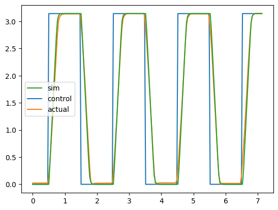
Plot of model vs collected data vs input signal.
Whoa, my guess was pretty good!
Discussion
Now let’s talk about why I am only varying $k_p$ and $b$ in my simulation.
I have made some close but imperfect guesses for $k_t$, $k_e$, and $R$, but let’s assume that our value for $G$ is correct. This gear ratio means that our servo hits its maximum velocity pretty quickly. This is often thought of as the servo’s “slew rate”. It is mostly a function of the gear ratio, the internal mechanical loss, back-emf constants, and driving voltage. Even if the guess for $k_e$ is too large, the internal damping lumped into $b$ can be increased to match what we see at the output. And just because we made a guess for $V_{supply}=5$, this will be wrong too, because the transistors driving the current across the motor’s coils will have a small voltage drop. Each of these unknowns serves to change the slope of the line; so we just have to pick one free variable to lump all these unknowns into. For this exercise I pick b, setting everything else to my educated guesswork from the datasheets, as discussed above.
Now let’s talk about $k_p$. Our servo is at its maximum speed throughout most of its motion, meaning that our controller is saturated. So where does $k_p$ play a role in the shape of our output? If you think about it, the controller is only unsaturated at the “knee” of the step function, near the corners, where the speed begins to finally drop as the error gets closer to zero. The magnitude of $k_p$ will thus only determine the sharpness of the corners of the step function.
Lets try a couple different values to see what I mean. Changing $k_p$ values results in a sharp or rounded transition near the corners of my actuator’s step response.
t,q1 = run_sim(kp = 2,b_act = b,render=False)
t,q2 = run_sim(kp = 4,b_act = b,render=False)
t,q3 = run_sim(kp = 20,b_act = b,render=False)

a1 = plt.plot(t_data,q1)
a2  = plt.plot(t_data,q2)
a3 = plt.plot(t_data,q3)
plt.legend(a1+a2+a3,['$k_p=2$','$k_p=4$','$k_p=20$'])
plt.show()
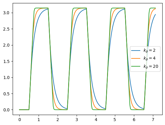
Comparing different values of $k_p$
Likewise, changing the damping value mostly impacts the slope.
t,q1 = run_sim(kp = 20,b_act = b,render=False)
t,q2 = run_sim(kp = 20,b_act = b*3,render=False)
t,q3 = run_sim(kp = 20,b_act = b*6,render=False)

a1 = plt.plot(t_data,q1)
a2  = plt.plot(t_data,q2)
a3 = plt.plot(t_data,q3)
plt.legend(a1+a2+a3,['$b={b:1.2e}$'.format(b=b),'$b={b:1.2e}$'.format(b=b*3),'$b={b:1.2e}$'.format(b=b*6)])
plt.show()
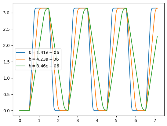
Comparing different values of $b$
Part 6: Parameter identification
So let’s find the best values for $k_p$ and $b$. I import scipy.optimize and define a function that will be called by the minimize function. It runs the simulation and compares the simulation data against the experimental data, finds the error, and returns the sum of squared error over time.
import scipy.optimize as so

def fun(vars):

    k,b = vars
    t,q = run_sim(k,b)


    error = q-q_data
    error = error**2
    error = error.sum()
    error = error**.5
    print(k,b,error)
    return error
test it with an initial guess. The error from my guess is ~1.46. Try other values, see what you can get!
ini = [15,b]
fun(ini)
15 1.4091678782734167e-06 1.458970807257259


1.458970807257259
I found many of the algorithms had trouble converging. I had to add bounds and play with the tolerances
results = so.minimize(fun,x0=ini,method='nelder-mead',bounds = ((1,100),(b*.1,b*10)),options={'xatol':1e-2,'fatol':1e-2})
15.0 1.4091678782734167e-06 1.458970807257259
15.75 1.4091678782734167e-06 1.462402830106116
15.0 1.4796262721870876e-06 1.4584701719279918
14.25 1.4796262721870876e-06 1.4562260034240078
13.5 1.514855469143923e-06 1.47061259159179
... ... ...
8.896713022899348 1.4041787991974594e-06 1.435694270256341
Check the final error. Better than when I started!
print(results)
       message: Optimization terminated successfully.
       success: True
        status: 0
           fun: 1.435694270256341
             x: [ 8.897e+00  1.404e-06]
           nit: 30
          nfev: 53
 final_simplex: (array([[ 8.897e+00,  1.404e-06],
                       [ 8.892e+00,  1.404e-06],
                       [ 8.890e+00,  1.404e-06]]), array([ 1.436e+00,  1.436e+00,  1.436e+00]))
Now run my simulation with the results of the optimization
t,q = run_sim(*results.x,render=True,video_filename='output.mp4')
Plot the results
a2 = plt.plot(t_data,desired)
a3  = plt.plot(t_data,q_data)
a1 = plt.plot(t_data,q)
plt.legend(a1+a2+a3,['sim','control','actual'])
plt.show()
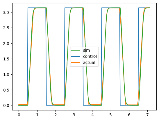
Comparing model fit vs experimental data and input signal.
Conclusions
As you can see, I was able to achieve a fairly good fit. Keep in mind, the values I found will probably stray a bit if you use the servo at a different supply voltages. But the fit I was able to achieve seems pretty good for estimating servo performance going forward. This model is not good for estimating the electrical efficiency, though, because our guesses for $k_e$ were not really validated or measured, and the true internal losses are not known. Without a power meter on the electrical side, I won’t be able to understand how much electrical energy it takes to achieve the motion I observed.
For the purposes of understanding the ability of our motors to generate mechanical power, though this model works.
External References
I used the following resources in the last two articles
- https://www.princeton.edu/~mae412/TEXT/NTRAK2002/292-302.pdf
- https://www.auselectronicsdirect.com.au/assets/brochures/TA0132.pdf
- https://components101.com/sites/default/files/component_datasheet/SG90%20Servo%20Motor%20Datasheet.pdf
- https://www.researchgate.net/publication/353754375
- https://www.kjell.com/globalassets/mediaassets/701916_87897_datasheet_en.pdf?ref=4287817A7A
- https://www.mpja.com/download/31002md%20data.pdf
- http://www.ee.ic.ac.uk/pcheung/teaching/DE1_EE/stores/sg90_datasheet.pdf