Inverse Dynamics in Mujoco

Introduction

This tutorial shows you how to use MuJoCo to compute the required torques to achieve a given directory. The example compares the computed torque from two different integrators.

If you have a model, inverse dynamics are a great way to compute most of the torques required to make your robot move along a particular trajectory. What we see from this example, though, is that if there is error – due to a poorly-selected integrator or too large of a time step – the computed torque does not capture the actual, underlying dynamics. This can have big implications if you want to control your robot with a feed-forward term that has noise, latency, etc.

import os
import mujoco
import numpy
import mediapy as media
import matplotlib.pyplot as plt
import math
import yaml
import scipy.interpolate

We create an xml template in python and then format it. We replace the ts variable with .001 initially it keeps the xml in the script so there are not extra files floating around.

xml_template = """
<mujoco>
  <option timestep="{ts:e}"/>
  <option integrator="{integrator}"/>
    <worldbody>
        <light name="top" pos="0 0 1"/>
        <body name="A" pos="0 0 0">
            <joint name="j1" type="hinge" axis="0 1 0" pos="0 0 0"/>
            <geom type="box" size=".5 .05 .05" pos=".5 0 0" rgba="1 0 0 1" mass="1"/>
            <body name="B" pos="1 0 0">
                <joint name="j2" type="hinge" axis="0 1 0" pos="0 0 0"/>
                <geom type="box" size=".5 .05 .05" pos=".5 0 0" rgba="1 0 0 1" mass="1"/>
            </body>
        </body>
    </worldbody>
    <actuator>
        <general name="m1" joint="j1"/>
        <general name="m2" joint="j2"/>
    </actuator>

</mujoco>
"""
xml = xml_template.format(ts=1e-3,integrator='RK4')

We load our model, data, and renderer from the xml

model = mujoco.MjModel.from_xml_string(xml)
data = mujoco.MjData(model)
renderer = mujoco.Renderer(model)

I create a simple controller that adds torque to the two joints using a sinusoidal curve.

freq = 1
def my_controller(model, data):
    theta1 = math.sin(2*math.pi*(freq*data.time))
    theta2 = math.sin(2*math.pi*(freq*data.time-.25))
    data.ctrl = [theta1,theta2]
    return

We run the simulation in order to obtain the system’s state as a function of time.

mujoco.mj_resetData(model,data)

duration = 3
framerate =30

q = []
w = []
a = []
t = []
xy = []
frames = []

try:
    mujoco.set_mjcb_control(my_controller)
    while data.time<duration:

        mujoco.mj_step(model,data)

        q.append(data.qpos.copy())
        w.append(data.qvel.copy())
        a.append(data.qacc.copy())
        xy.append(data.xpos.copy())
        t.append(data.time)
        
        if len(frames)<data.time*framerate:
        
            renderer.update_scene(data)
            # renderer.update_scene(data,"world")
            pixels = renderer.render()
            frames.append(pixels)
finally:
    mujoco.set_mjcb_control(None)
        
media.show_video(frames,fps = framerate)

Convert the obtained values into arrays

q = numpy.array(q)
w = numpy.array(w)
a = numpy.array(a)
xy = numpy.array(xy)
t = numpy.array(t)

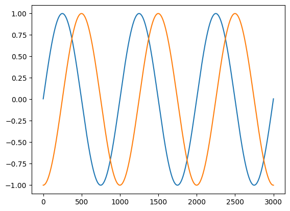
plt.plot(t,q)

[<matplotlib.lines.Line2D at 0x7523418e49d0>,
 <matplotlib.lines.Line2D at 0x75233cf8d110>]

Reset the model to the same starting condition and substitute each position, velocity, and acceleration term into the state for each time, and use the data.qfrc_inverse function to evaluate the required joint torques…then append these to a list

mujoco.mj_resetData(model,data)
torque_est = []

for q_ii,w_ii,a_ii in zip(q,w,a):
    data.qpos[:] = q_ii
    data.qvel[:] = w_ii
    data.qacc[:] = a_ii
    mujoco.mj_inverse(model,data)
    torque =  data.qfrc_inverse.copy()
    torque_est.append(torque)

torque_est = numpy.array(torque_est)

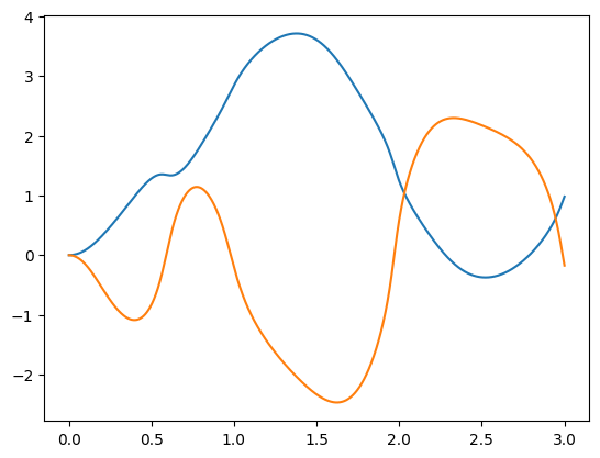
Plot the resulting torques.

plt.plot(torque_est)

[<matplotlib.lines.Line2D at 0x75231b701d90>,
 <matplotlib.lines.Line2D at 0x75231b73b350>]

This works great for data at 1000 Hz, but what if our simulation had been run at a slower speed or with a different integrator? First we create a function that runs the sim with different parameters

def run_model(controller,**kwargs):
    xml = xml_template.format(**kwargs)
    model = mujoco.MjModel.from_xml_string(xml)
    data = mujoco.MjData(model)
    mujoco.mj_resetData(model,data)
    
    duration = 3
    framerate =30
    
    q2 = []
    w2 = []
    a2 = []
    t2 = []
    xy2 = []
    
    try:
        mujoco.set_mjcb_control(controller)
        while data.time<duration:
    
            mujoco.mj_step(model,data)
    
            q2.append(data.qpos.copy())
            w2.append(data.qvel.copy())
            a2.append(data.qacc.copy())
            xy2.append(data.xpos.copy())
            t2.append(data.time)
    finally:
        mujoco.set_mjcb_control(None)
    
    q2 = numpy.array(q2)
    w2 = numpy.array(w2)
    a2 = numpy.array(a2)
    xy2 = numpy.array(xy2)
    t2 = numpy.array(t2)
    return model,data,q2,w2,a2,xy2,t2

Now we run with a different integrator

model,data,q2,w2,a2,xy2,t2 = run_model(my_controller,ts=1e-3,integrator='Euler')

plt.plot(t2,q2)

[<matplotlib.lines.Line2D at 0x75231b779210>,
 <matplotlib.lines.Line2D at 0x752340da1e10>]

Though the motion looks nearly the same as before, there are small differences, and they grow with time:

y=plt.plot(t,q-q2)

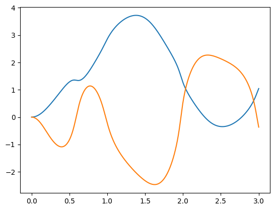
The inverse dynamics begin look worse too:

def calc_torque(model,data,q2,w2,a2):
    torque_est2 = []
    
    for q_ii,w_ii,a_ii in zip(q2,w2,a2):
        data.qpos[:] = q_ii
        data.qvel[:] = w_ii
        data.qacc[:] = a_ii
        mujoco.mj_inverse(model,data)
        torque =  data.qfrc_inverse.copy()
        torque_est2.append(torque)
    
    torque_est2 = numpy.array(torque_est2)
    return torque_est2

torque_est2 = calc_torque(model,data,q2,w2,a2)
plt.plot(torque_est2)

[<matplotlib.lines.Line2D at 0x75231b65af90>,
 <matplotlib.lines.Line2D at 0x75231b176f90>]

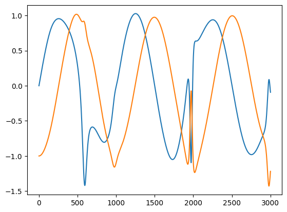
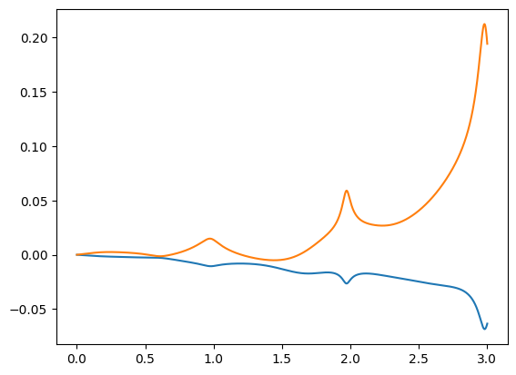
And when applied back to the original model, there is quite a difference. First we create an interpolation function, and use that to supply a torque command at a time t

f = scipy.interpolate.interp1d(t2,torque_est2.T,fill_value=(t2[0],t2[-1]), bounds_error=False,)

def my_controller2(model, data):
    torque = f(data.time)
    data.ctrl = [*torque]
    return

model,data,q3,w3,a3,xy3,t3 = run_model(my_controller2,ts=1e-3,integrator='RK4')
plt.plot(q3-q)

[<matplotlib.lines.Line2D at 0x75231b1c5fd0>,
 <matplotlib.lines.Line2D at 0x75231b026f90>]

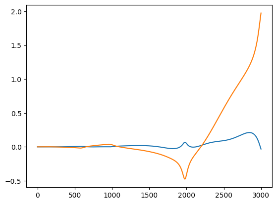
What does this mean? Even with small position errors due to the wrong integration scheme or large time-steps, our computed torque starts to diverge from the torques required to acurately achieve a desired trajectory. Thus, if we are doing inverse dynamics, we need to correct for those growing losses by adding a controller.