Introduction

The purpose of this tutorial is to show you the power of sympy for analyzing the math of linkages and kinematics. We will walk through a full example of solving for the motion of a four-bar linkage, with a variety of approaches explored along the way with an eye towards addressing sympy’s limitations, compared to other symbolic math environments like Mathematica, Maple, etc.

First, import all your libraries. Note that we want to use the symbolic form of sin and cos a lot, so we intentionally import those functions into our main namespace. Likewise, we want to use the numeric value of pi often, so we can import that directly from the math package.

import sympy
from sympy import sin,cos
import math
from math import pi
import numpy
import scipy
import matplotlib.pyplot as plt
import scipy.optimize as so

You can create multiple symbols at a time, with latex formatting. if you want to use the backslash, however, remember that the backslash in Python is used for non-printing characters like \n and \t. Therefore, to “escape” that default, you have to use two backslashes. What would normally be \theta in latex should be \\theta in a Python string.

Separate your separate symbols in the string with spaces or commas, and make sure each one has its own Python variable that it is saved to.

qa,qb,qc,qd = sympy.symbols('\\theta_a,\\theta_b,\\theta_c,\\theta_d')
la,lb,lc,ld = sympy.symbols('l_a,l_b,l_c,l_d')

We can test what was produced to see how it formats in a Jupyter notebook. Pretty!

qa

$\displaystyle \theta_{a}$

Next, we define a function to create rotation matrices with the rotation about the z axis. We are doing a planar example, so we only need a $R_z$ matrices. The function allows us to generate multiple rotation matrices, with different variables controlling the rotation amount, using the same code. Efficient!

def Rz(theta):
    Rz = sympy.Matrix([[cos(theta),-sin(theta),0],[sin(theta),cos(theta),0],[0,0,1]])
    return Rz

Ra = Rz(qa)
Rb = Rz(qb)
Rc = Rz(qc)
Rd = Rz(qd)

Ra

$\displaystyle \left[\begin{matrix}\cos{\left(\theta_{a} \right)} & - \sin{\left(\theta_{a} \right)} & 0 \\ \sin{\left(\theta_{a} \right)} & \cos{\left(\theta_{a} \right)} & 0 \\ 0 & 0 & 1\end{matrix}\right]$

Next, create a Cartesian unit vector in the x direction. This is a generic unit vector variable that is not associated with any frame, so we can just call it x

x = sympy.Matrix([1,0,0])
x

$\displaystyle \left[\begin{matrix}1\\0\\0\end{matrix}\right]$

Now, let’s create a vector $\vec{v}_1$, defined as the length of the A link, along the x-axis in the A frame. We need to transform it into the N frame (our base frame) in order to relate it to other vectors.

v1_in_A = (la*x)
v1_in_N = Ra*v1_in_A
v1_in_N

$\displaystyle \left[\begin{matrix}l_{a} \cos{\left(\theta_{a} \right)}\\l_{a} \sin{\left(\theta_{a} \right)}\\0\end{matrix}\right]$

We can use a dictionary to substitute numerical values for the symbolic variables. This is useful for plotting and solving specific problems

v1_in_N.subs({qa:91*pi/180,la:1})

$\displaystyle \left[\begin{matrix}-0.0174524064372835\\0.999847695156391\\0\end{matrix}\right]$

We can now define the remaining vectors of the four-bar in the same way. $\vec{v}_2$ is the distance along link B, from the end of link A. Its rotation is relative to the rotation of link A. Therefore, to express it in the N(base) frame, we need to express it first in terms of A, then N.

v2_in_B = lb*x
v2_in_A = Rb*v2_in_B
v2_in_N = Ra*v2_in_A
v2_in_N

$\displaystyle \left[\begin{matrix}- l_{b} \sin{\left(\theta_{a} \right)} \sin{\left(\theta_{b} \right)} + l_{b} \cos{\left(\theta_{a} \right)} \cos{\left(\theta_{b} \right)}\\l_{b} \sin{\left(\theta_{a} \right)} \cos{\left(\theta_{b} \right)} + l_{b} \sin{\left(\theta_{b} \right)} \cos{\left(\theta_{a} \right)}\\0\end{matrix}\right]$

$\vec{v}_3$ represents link C. It rotates relative to the base frame.

v3_in_C = lc*x
v3_in_N = Rc*v3_in_C
v3_in_N

$\displaystyle \left[\begin{matrix}l_{c} \cos{\left(\theta_{c} \right)}\\l_{c} \sin{\left(\theta_{c} \right)}\\0\end{matrix}\right]$

Like link B, link D rotates relative to link C. $\vec{v}_4$ represents link D, and it needs to be expressed first in C, and then in N, in order to relate it to other vectors

v4_in_D = ld*x
v4_in_C = Rd*v4_in_D
v4_in_N = Rc*v4_in_C
v4_in_N

$\displaystyle \left[\begin{matrix}- l_{d} \sin{\left(\theta_{c} \right)} \sin{\left(\theta_{d} \right)} + l_{d} \cos{\left(\theta_{c} \right)} \cos{\left(\theta_{d} \right)}\\l_{d} \sin{\left(\theta_{c} \right)} \cos{\left(\theta_{d} \right)} + l_{d} \sin{\left(\theta_{d} \right)} \cos{\left(\theta_{c} \right)}\\0\end{matrix}\right]$

$\vec{v}_1$,$\vec{v}_2$,$\vec{v}_3$, and $\vec{v}_4$ are all relative vectors relating the positon of the end-effector of their links from their origin. To express their absolute position, we define $\vec{p}_1$ - $\vec{p}_4$ to express the absolute position of each joint in global space. The position of these points is all related to some origin point, $\vec{o}$ which we also define.

o = sympy.Matrix([0,0,0])
p1 = o+v1_in_N
p2 = o+p1+v2_in_N
p3 = o+v3_in_N
p4 = o+p3+v4_in_N

Assembling each point permits us to plot the mechanism. We create a variable called points, which holds a list of each point in a particular order convenient for plotting (between each of the points listed, we want to draw a line).

points = sympy.Matrix([p2.T,p1.T,o.T,p3.T,p4.T]).T
points

$\displaystyle \left[\begin{matrix}l_{a} \cos{\left(\theta_{a} \right)} - l_{b} \sin{\left(\theta_{a} \right)} \sin{\left(\theta_{b} \right)} + l_{b} \cos{\left(\theta_{a} \right)} \cos{\left(\theta_{b} \right)} & l_{a} \cos{\left(\theta_{a} \right)} & 0 & l_{c} \cos{\left(\theta_{c} \right)} & l_{c} \cos{\left(\theta_{c} \right)} - l_{d} \sin{\left(\theta_{c} \right)} \sin{\left(\theta_{d} \right)} + l_{d} \cos{\left(\theta_{c} \right)} \cos{\left(\theta_{d} \right)}\\l_{a} \sin{\left(\theta_{a} \right)} + l_{b} \sin{\left(\theta_{a} \right)} \cos{\left(\theta_{b} \right)} + l_{b} \sin{\left(\theta_{b} \right)} \cos{\left(\theta_{a} \right)} & l_{a} \sin{\left(\theta_{a} \right)} & 0 & l_{c} \sin{\left(\theta_{c} \right)} & l_{c} \sin{\left(\theta_{c} \right)} + l_{d} \sin{\left(\theta_{c} \right)} \cos{\left(\theta_{d} \right)} + l_{d} \sin{\left(\theta_{d} \right)} \cos{\left(\theta_{c} \right)}\\0 & 0 & 0 & 0 & 0\end{matrix}\right]$

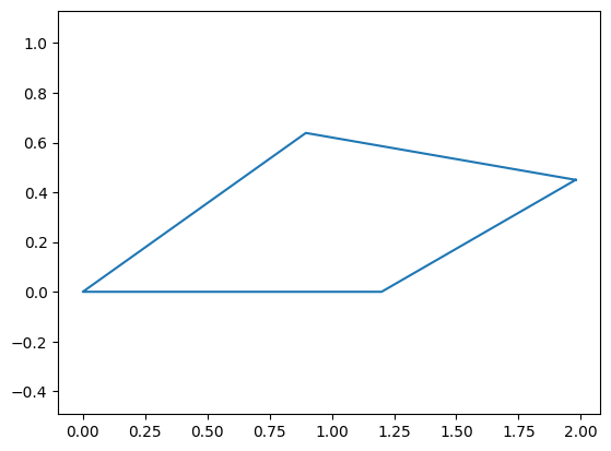
We now want to plot the mechansim. We define two variables: design and state. Design is intended to hold all our … “design” variables and you guessed it, state holds our “state” variables. Because we have, so far, a serial mechanism, all the rotations define the state of this open chain.

design = {la:1.2,lb:.9,lc:1.1,ld:1.1}
state = {qa:0*pi/180,qb:30*pi/180,qc:45*pi/180,qd:-30*pi/180}

We substitute our design and state variables into points and plot the x and y coordinates

points_n = points.subs({**design,**state})
points_n = numpy.array(points_n,dtype = numpy.float64)
plt.plot(*points_n[:2])
plt.axis('equal')

(-0.09897114317029974,
 2.0783940065762945,
 -0.053125920445898756,
 1.1156443293638738)

Solving closed loop constraints

We would now like to use these expressions to solve for a valid configuration where the four-bar linkage is closed. This means that $\vec{p}_2$ and $\vec{p}_4$ are located at the same spot. In general, we can create a constraint equation that represents that condition, and then solve for our remaining free variables in order to find a valid configuration. First we define our expression:

$$\vec{p}_2=\vec{p}_4$$

This useful for written math, but using sympy we need to eliminate the equals sign. Thus, we rewrite it as

$$0=\vec{p}_4-\vec{p}_2$$

and create a variable zero that holds this equation’s right hand side, truncating the trivial z-axis information:

zero = p4-p2
zero = sympy.Matrix(zero[:2])
zero

$\displaystyle \left[\begin{matrix}- l_{a} \cos{\left(\theta_{a} \right)} + l_{b} \sin{\left(\theta_{a} \right)} \sin{\left(\theta_{b} \right)} - l_{b} \cos{\left(\theta_{a} \right)} \cos{\left(\theta_{b} \right)} + l_{c} \cos{\left(\theta_{c} \right)} - l_{d} \sin{\left(\theta_{c} \right)} \sin{\left(\theta_{d} \right)} + l_{d} \cos{\left(\theta_{c} \right)} \cos{\left(\theta_{d} \right)}\\- l_{a} \sin{\left(\theta_{a} \right)} - l_{b} \sin{\left(\theta_{a} \right)} \cos{\left(\theta_{b} \right)} - l_{b} \sin{\left(\theta_{b} \right)} \cos{\left(\theta_{a} \right)} + l_{c} \sin{\left(\theta_{c} \right)} + l_{d} \sin{\left(\theta_{c} \right)} \cos{\left(\theta_{d} \right)} + l_{d} \sin{\left(\theta_{d} \right)} \cos{\left(\theta_{c} \right)}\end{matrix}\right]$

We now need to define some other variables. First, we need to “fix” the base of the four-bar linkage. In the case of this four-bar, it makes sense to define the A link as fixed to the ground, with $\theta_a=0$. Thus, we move qa into our list of “design” variables rather than state variables, since it never changes in our analysis

design = {qa:0,**design}
design

{\theta_a: 0, l_a: 1.2, l_b: 0.9, l_c: 1.1, l_d: 1.1}

We now substitute our design variables into zero to create a specific case of our solution.

zero_specific=zero.subs(design)
zero_specific = sympy.Matrix(zero_specific)
zero_specific

$\displaystyle \left[\begin{matrix}- 1.1 \sin{\left(\theta_{c} \right)} \sin{\left(\theta_{d} \right)} - 0.9 \cos{\left(\theta_{b} \right)} + 1.1 \cos{\left(\theta_{c} \right)} \cos{\left(\theta_{d} \right)} + 1.1 \cos{\left(\theta_{c} \right)} - 1.2\\- 0.9 \sin{\left(\theta_{b} \right)} + 1.1 \sin{\left(\theta_{c} \right)} \cos{\left(\theta_{d} \right)} + 1.1 \sin{\left(\theta_{c} \right)} + 1.1 \sin{\left(\theta_{d} \right)} \cos{\left(\theta_{c} \right)}\end{matrix}\right]$

how many variables still exist in these equations? we can use the .atoms() method to find out

zero_specific.atoms(sympy.Symbol)

{\theta_b, \theta_c, \theta_d}

But we have only two nontrivial equations and three unknowns! How do we solve for all three? Well, this helps us understand how many degrees of freedom exist in this system. One of these variables is a free parameter (also known as an independent variable), which we can select. The other two are dependent variables, which are determined by the independent variable. Let’s supply our independent variable so that the remaining equations can be solved. Let’s pick $\theta_b$

independent={qb:120*pi/180}
zero_specific=zero_specific.subs(independent)
zero_specific

$\displaystyle \left[\begin{matrix}- 1.1 \sin{\left(\theta_{c} \right)} \sin{\left(\theta_{d} \right)} + 1.1 \cos{\left(\theta_{c} \right)} \cos{\left(\theta_{d} \right)} + 1.1 \cos{\left(\theta_{c} \right)} - 0.75\\1.1 \sin{\left(\theta_{c} \right)} \cos{\left(\theta_{d} \right)} + 1.1 \sin{\left(\theta_{c} \right)} + 1.1 \sin{\left(\theta_{d} \right)} \cos{\left(\theta_{c} \right)} - 0.779422863405995\end{matrix}\right]$

Numerical Solving process

We are first going to use a numerical approach to solving this problem, using the scipy.optimize package.

We now want to provide an initial guess for our two remaining dependent variables, $\theta_c$ and $\theta_d$, and a function that calculates the error of a guess for $\theta_c$ and $\theta_d$. We do this by supplying zero with a guess for $\theta_c$ and $\theta_d$, and computing the sum of squared error on the “residual”. Residual basically means the error between our computed answer and what it should be, 0.

ini = [45*math.pi/180,-45*math.pi/180]

def myfun(guess):
    qc_guess,qd_guess = guess
    zero_guess = zero_specific.subs({qc:qc_guess,qd:qd_guess})
    zero_guess_n = numpy.array(zero_guess,dtype = numpy.float64)
    sum_of_squared_error = ((zero_guess_n**2).sum())**.5        
    # print(guess,sum_of_squared_error)
    return sum_of_squared_error

we now supply our guess and function to the scipy.optimize.minimize() function, which can be used to identify the guess for $\theta_c$ and $\theta_d$ that minimizes the error

res = so.minimize(myfun,ini,method="powell")
res

 message: Optimization terminated successfully.
 success: True
  status: 0
     fun: 3.2518256220118898e-12
       x: [ 1.861e+00 -2.114e+00]
     nit: 7
   direc: [[ 0.000e+00  1.000e+00]
           [ 1.524e-01 -6.886e-02]]
    nfev: 297

Within the result we see a couple things. First, we see if the optimization process was successful. It says so. Second, we see res.fun, which indicates the magnitude of the residual error after our final guess, which is incredibly small. Finally, we see res.x, indicating the solution the solver found. We insert x into a dictionary

dependent = dict(zip([qc,qd],res.x))

and plot:

points_n = points.subs({**design,**independent,**dependent})
points_n = numpy.array(points_n,dtype = numpy.float64)
plt.plot(*points_n[:2])
plt.axis('equal')

(-0.390973836659514,
 1.2757606588885482,
 -0.052693468583865546,
 1.1065628402611765)

But what if we want to find the solution using a different design, or different value for our independent variable? We need to generate a different function before solving. We can do this by wrapping function generation within another function.

def gen_fun(design,independent):
    zero_specific = zero.subs({**design,**independent})
    zero_specific = sympy.Matrix(zero_specific[:2])

    def fun(guess):
        qc_guess,qd_guess = guess
        zero_guess = zero_specific.subs({qc:qc_guess,qd:qd_guess})
        zero_guess_n = numpy.array(zero_guess,dtype = numpy.float64)
        sum_of_squared_error = ((zero_guess_n**2).sum())**.5        
        # print(guess,sum_of_squared_error)
        return sum_of_squared_error
    
    return fun

Let’s also make a function for plotting.

def plot_fourbar(design,independent,dependent):
    points_n = points.subs({**design,**independent,**dependent})
    points_n = numpy.array(points_n,dtype = numpy.float64)
    plt.plot(*points_n[:2])
    plt.axis('equal')

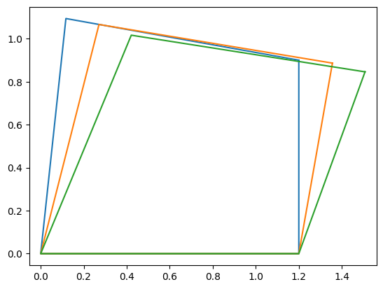
Now, we can supply different points and plot them

ini = [45*math.pi/180,-45*math.pi/180]

independent = {qb:90*pi/180}
myfun = gen_fun(design,independent)
res = so.minimize(myfun,ini)
dependent = dict(zip([qc,qd],res.x))      
plot_fourbar(design,independent,dependent)

independent = {qb:80*pi/180}
myfun = gen_fun(design,independent)
res = so.minimize(myfun,ini)
dependent = dict(zip([qc,qd],res.x))      
plot_fourbar(design,independent,dependent)

independent = {qb:70*pi/180}
myfun = gen_fun(design,independent)
res = so.minimize(myfun,ini)
dependent = dict(zip([qc,qd],res.x))      
plot_fourbar(design,independent,dependent)

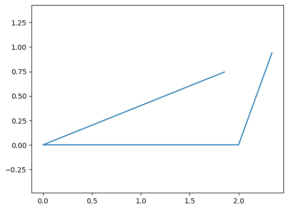
The problem is that the solver can sometimes fail, or converge to an unexpected answer This can be for a couple reasons.

1. You supplied a bad initial guess
2. There is no solution given the combination of design parameters and independent parameters you selected.

For example:

ini = [45*math.pi/180,-45*math.pi/180]
design = {qa:0,la:2,lb:1,lc:1,ld:1}
independent = {qb:70*pi/180}

myfun = gen_fun(design,independent)
res = so.minimize(myfun,ini)
dependent = dict(zip([qc,qd],res.x))      
plot_fourbar(design,independent,dependent)

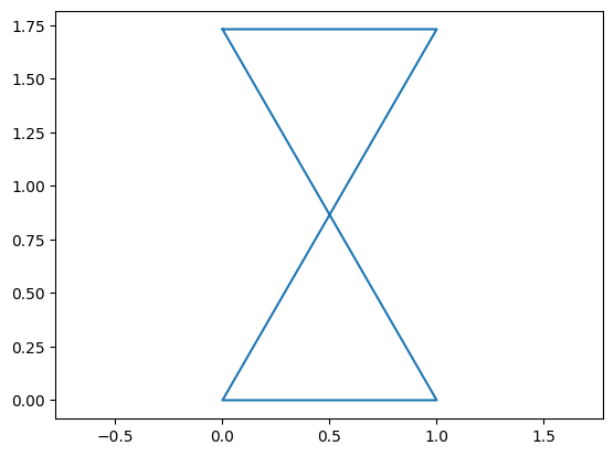
ini = [45*math.pi/180,90*math.pi/180]
design = {qa:0,la:1,lb:2,lc:2,ld:1}
independent = {qb:120*pi/180}

myfun = gen_fun(design,independent)
res = so.minimize(myfun,ini)
dependent = dict(zip([qc,qd],res.x))      
plot_fourbar(design,independent,dependent)

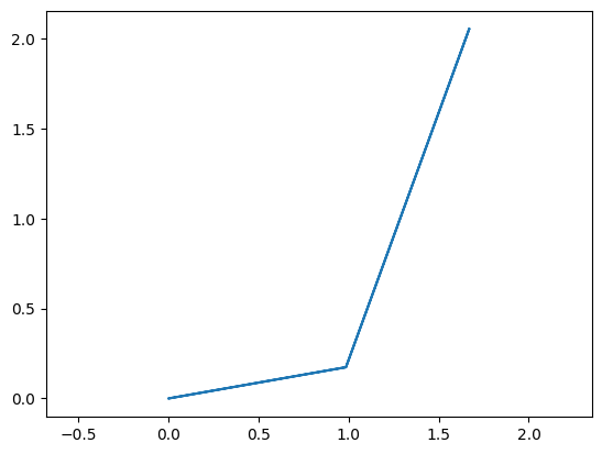
ini = [10*math.pi/180,60*math.pi/180]
design = {qa:10*pi/180,la:1,lb:2,lc:1,ld:2}
independent = {qb:60*pi/180}

myfun = gen_fun(design,independent)
res = so.minimize(myfun,ini)
dependent = dict(zip([qc,qd],res.x))      
plot_fourbar(design,independent,dependent)

Symbolic Solving

So how can we solve the symbolic expressions directly? Well we can use sympy.solve(). For example, we can take a specific design in a specific state, and solve for the remaining variables:

design = {qa:0,la:1.2,lb:.9,lc:1.1,ld:1.1}
independent = {qb:30*pi/180}
zero_specific = zero.subs({**design,**independent})
zero_specific

$\displaystyle \left[\begin{matrix}- 1.1 \sin{\left(\theta_{c} \right)} \sin{\left(\theta_{d} \right)} + 1.1 \cos{\left(\theta_{c} \right)} \cos{\left(\theta_{d} \right)} + 1.1 \cos{\left(\theta_{c} \right)} - 1.97942286340599\\1.1 \sin{\left(\theta_{c} \right)} \cos{\left(\theta_{d} \right)} + 1.1 \sin{\left(\theta_{c} \right)} + 1.1 \sin{\left(\theta_{d} \right)} \cos{\left(\theta_{c} \right)} - 0.45\end{matrix}\right]$

sol = sympy.solve(zero_specific,(qc,qd))
sol

[(-0.172242420242400, 0.791564062543542),
 (0.619321642301143, -0.791564062543542)]

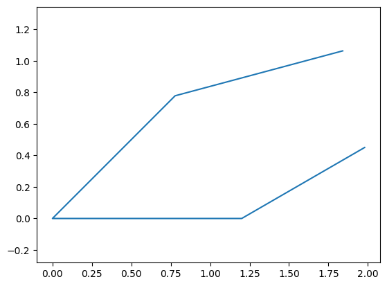
The solver was successfully able to identify the two potential solutions to the trigonometric problem:

dependent = dict(zip([qc,qd],sol[0]))      
plt.figure()
plot_fourbar(design,independent,dependent)
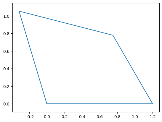
dependent = dict(zip([qc,qd],sol[1]))      
plt.figure()
plot_fourbar(design,independent,dependent)

But we had already substituted all the other symbolic variables with numeric answers. What if we wanted to solve the generic problem as a function of qb?

design = {qa:0,la:1.2,lb:.9,lc:1.1,ld:1.1}
# zero = sympy.Matrix((p4-p2)[:2])
zero_specific = zero.subs(design)
zero_specific

$\displaystyle \left[\begin{matrix}- 1.1 \sin{\left(\theta_{c} \right)} \sin{\left(\theta_{d} \right)} - 0.9 \cos{\left(\theta_{b} \right)} + 1.1 \cos{\left(\theta_{c} \right)} \cos{\left(\theta_{d} \right)} + 1.1 \cos{\left(\theta_{c} \right)} - 1.2\\- 0.9 \sin{\left(\theta_{b} \right)} + 1.1 \sin{\left(\theta_{c} \right)} \cos{\left(\theta_{d} \right)} + 1.1 \sin{\left(\theta_{c} \right)} + 1.1 \sin{\left(\theta_{d} \right)} \cos{\left(\theta_{c} \right)}\end{matrix}\right]$

In this case we supplied all the design variables but did not include the independent parameter. The expressions don’t look too hard…should we try solving?

NO!

Unfortunately, sympy is not able to solve this expression as a function of the independent variable in a reasonable time. This is both due to sympy’s limitations, and due to the fact that the nested trigonometric functions hide quite a bit of complexity. So don’t run the code below: generic_solution = sympy.solve(zero_specific,(qc,qd)) So now let’s try to simplify the expression by hand a little bit. First thing to recognize is that the coupler of our four-bar (link D) can be removed from the expression. Instead of saying that $\vec{p}_4-\vec{p}_2=0$, we could also say that $$|\vec{p}_3 - \vec{p}_2|=l_d$$ This permits us to remove $q_d$ entirely from the set of equations, simplifying our expression to $$(\vec{p}_3 - \vec{p}_2)\cdot (\vec{p}_3 - \vec{p}_2) = l_d$$ in sympy,

coupler = p3-p2
zero2 = (coupler.T*coupler)[0]-ld**2
zero2
zero_specific = zero2.subs(design)
zero_specific

$\displaystyle 1.21 \left(- 0.818181818181818 \sin{\left(\theta_{b} \right)} + \sin{\left(\theta_{c} \right)}\right)^{2} + 1.44 \left(- 0.75 \cos{\left(\theta_{b} \right)} + 0.916666666666667 \cos{\left(\theta_{c} \right)} - 1\right)^{2} - 1.21$

Not too bad…but again, the squares hide some complexity. What does it look like when we expand this expression?

zero_specific = zero_specific.expand()
zero_specific

$\displaystyle 0.81 \sin^{2}{\left(\theta_{b} \right)} - 1.98 \sin{\left(\theta_{b} \right)} \sin{\left(\theta_{c} \right)} + 1.21 \sin^{2}{\left(\theta_{c} \right)} + 0.81 \cos^{2}{\left(\theta_{b} \right)} - 1.98 \cos{\left(\theta_{b} \right)} \cos{\left(\theta_{c} \right)} + 2.16 \cos{\left(\theta_{b} \right)} + 1.21 \cos^{2}{\left(\theta_{c} \right)} - 2.64 \cos{\left(\theta_{c} \right)} + 0.23$

Oof, getting longer. Let’s use the simplify expression to try to identify ways of eliminating redundancies, using trig identities to shorten the expression, etc.

zero_specific = zero_specific.simplify()
zero_specific

$\displaystyle 2.16 \cos{\left(\theta_{b} \right)} - 2.64 \cos{\left(\theta_{c} \right)} - 1.98 \cos{\left(\theta_{b} - \theta_{c} \right)} + 2.25$

Now it’s much shorter, but is it short enough for sympy to solve with respect to $\theta_b$? Unfortunately no. Don’t run the next command: generic_solution = sympy.solve(zero_specific,(qc))

General Solution

Okay, so how to do this, while capturing all the variables of the design? We have to help sympy. First, let’s only supply the definition for $\theta_a$ to our zero2 variable:

zero_specific = zero2.subs({qa:0})
zero_specific

$\displaystyle - l_{d}^{2} + \left(- l_{b} \sin{\left(\theta_{b} \right)} + l_{c} \sin{\left(\theta_{c} \right)}\right)^{2} + \left(- l_{a} - l_{b} \cos{\left(\theta_{b} \right)} + l_{c} \cos{\left(\theta_{c} \right)}\right)^{2}$

Let’s expand to see how bad it is…

zero_specific = zero_specific.expand()
zero_specific

$\displaystyle l_{a}^{2} + 2 l_{a} l_{b} \cos{\left(\theta_{b} \right)} - 2 l_{a} l_{c} \cos{\left(\theta_{c} \right)} + l_{b}^{2} \sin^{2}{\left(\theta_{b} \right)} + l_{b}^{2} \cos^{2}{\left(\theta_{b} \right)} - 2 l_{b} l_{c} \sin{\left(\theta_{b} \right)} \sin{\left(\theta_{c} \right)} - 2 l_{b} l_{c} \cos{\left(\theta_{b} \right)} \cos{\left(\theta_{c} \right)} + l_{c}^{2} \sin^{2}{\left(\theta_{c} \right)} + l_{c}^{2} \cos^{2}{\left(\theta_{c} \right)} - l_{d}^{2}$

Ouch. Let’s simplify:

z2 = zero_specific.simplify()
z2

$\displaystyle l_{a}^{2} + 2 l_{a} l_{b} \cos{\left(\theta_{b} \right)} - 2 l_{a} l_{c} \cos{\left(\theta_{c} \right)} + l_{b}^{2} - 2 l_{b} l_{c} \cos{\left(\theta_{b} - \theta_{c} \right)} + l_{c}^{2} - l_{d}^{2}$

Better. This helped find $\sin^2(x) + \cos^2(x) = 1$ identities and eliminate them, as well as shorten trig expressions where possible. But our simplify did too much condensing, bringing $\theta_b$ and $\theta_c$ within a $cos()$ term. For our solver, this makes things harder again. Let’s expand back out:

z3=sympy.expand_trig(z2).expand()
z3

$\displaystyle l_{a}^{2} + 2 l_{a} l_{b} \cos{\left(\theta_{b} \right)} - 2 l_{a} l_{c} \cos{\left(\theta_{c} \right)} + l_{b}^{2} - 2 l_{b} l_{c} \sin{\left(\theta_{b} \right)} \sin{\left(\theta_{c} \right)} - 2 l_{b} l_{c} \cos{\left(\theta_{b} \right)} \cos{\left(\theta_{c} \right)} + l_{c}^{2} - l_{d}^{2}$

Now the tricky part. We see in this expanded form that $\theta_c$ comes either in the form of $\sin(\theta_c)$ and $\cos(\theta_c)$ terms. lets collect our expression around terms that contain those, or not.

d = z3.collect((sin(qc),cos(qc)),evaluate=False)
for key in d.keys():
    print(key,': ',d[key])

cos(\theta_c) :  -2*l_a*l_c - 2*l_b*l_c*cos(\theta_b)
sin(\theta_c) :  -2*l_b*l_c*sin(\theta_b)
1 :  l_a**2 + 2*l_a*l_b*cos(\theta_b) + l_b**2 + l_c**2 - l_d**2

Using some advanced features of the collect function, we see that all the terms of the expression are either multiplied by $\sin(\theta_c)$ and $\cos(\theta_c)$ or $1$. Since we are trying to solve for $\theta_c$, let’s substitute in simpler expressions for those coefficients.

First we create 3 new symbols, for the 3 sets of coefficients we are replacing

symbol_strings = ['s_{}'.format(ii) for ii in range(len(d))]
symbol_strings = ','.join(symbol_strings)
symbols = sympy.symbols(symbol_strings)
symbols

(s_0, s_1, s_2)

We then create two new dictionaries. z4_subs1 is going to hold our replacement symbols for the three coefficients

keys = d.keys()
z4_subs1 = dict(zip(keys,symbols))
z4_subs1

{cos(\theta_c): s_0, sin(\theta_c): s_1, 1: s_2}

The second dictionary will replace the symbols with the original coefficients, once we have solved.

z4_subs2 = dict(zip(symbols,[d[item] for item in keys]))
z4_subs2

{s_0: -2*l_a*l_c - 2*l_b*l_c*cos(\theta_b),
 s_1: -2*l_b*l_c*sin(\theta_b),
 s_2: l_a**2 + 2*l_a*l_b*cos(\theta_b) + l_b**2 + l_c**2 - l_d**2}

We create expression z4, which is each key ($\sin(\theta_c)$, $\cos(\theta_c)$, $1$) times our new symbols

z4 = [item*z4_subs1[item] for item in keys]
z4 = sum(z4)
z4

$\displaystyle s_{0} \cos{\left(\theta_{c} \right)} + s_{1} \sin{\left(\theta_{c} \right)} + s_{2}$

Aah, finally simple enough to solve

sol = sympy.solve(z4,qc)
sol = sympy.Matrix(sol)
sol

$\displaystyle \left[\begin{matrix}2 \operatorname{atan}{\left(\frac{s_{1} - \sqrt{s_{0}^{2} + s_{1}^{2} - s_{2}^{2}}}{s_{0} - s_{2}} \right)}\\2 \operatorname{atan}{\left(\frac{s_{1} + \sqrt{s_{0}^{2} + s_{1}^{2} - s_{2}^{2}}}{s_{0} - s_{2}} \right)}\end{matrix}\right]$

We now replace s_0, s_1, and s_2 with their original contents:

sol = sol.subs(z4_subs2)
sol

$\displaystyle \left[\begin{matrix}2 \operatorname{atan}{\left(\frac{- 2 l_{b} l_{c} \sin{\left(\theta_{b} \right)} - \sqrt{4 l_{b}^{2} l_{c}^{2} \sin^{2}{\left(\theta_{b} \right)} + \left(- 2 l_{a} l_{c} - 2 l_{b} l_{c} \cos{\left(\theta_{b} \right)}\right)^{2} - \left(l_{a}^{2} + 2 l_{a} l_{b} \cos{\left(\theta_{b} \right)} + l_{b}^{2} + l_{c}^{2} - l_{d}^{2}\right)^{2}}}{- l_{a}^{2} - 2 l_{a} l_{b} \cos{\left(\theta_{b} \right)} - 2 l_{a} l_{c} - l_{b}^{2} - 2 l_{b} l_{c} \cos{\left(\theta_{b} \right)} - l_{c}^{2} + l_{d}^{2}} \right)}\\2 \operatorname{atan}{\left(\frac{- 2 l_{b} l_{c} \sin{\left(\theta_{b} \right)} + \sqrt{4 l_{b}^{2} l_{c}^{2} \sin^{2}{\left(\theta_{b} \right)} + \left(- 2 l_{a} l_{c} - 2 l_{b} l_{c} \cos{\left(\theta_{b} \right)}\right)^{2} - \left(l_{a}^{2} + 2 l_{a} l_{b} \cos{\left(\theta_{b} \right)} + l_{b}^{2} + l_{c}^{2} - l_{d}^{2}\right)^{2}}}{- l_{a}^{2} - 2 l_{a} l_{b} \cos{\left(\theta_{b} \right)} - 2 l_{a} l_{c} - l_{b}^{2} - 2 l_{b} l_{c} \cos{\left(\theta_{b} \right)} - l_{c}^{2} + l_{d}^{2}} \right)}\end{matrix}\right]$

This is finally a general solution to our coupler problem, but it takes a while to run the .subs() function within a loop. We can use the sympy.lambdify() function to turn this expression into a function, which is generally faster to evaluate. To do this we need to supply all the variables we need to replace in this expression to the lambdify function. We can use the atoms() function again to find them:

variables = list(sol[0].atoms(sympy.Symbol))
variables

[\theta_b, l_c, l_d, l_b, l_a]

We then “lambdify” the solution:

fc = sympy.lambdify(variables,sol)

And now we can use it with a given design and state

design = {qa:0,la:1,lb:1,lc:1,ld:.7}
independent = {qb:120*pi/180}
input = [{**design,**independent}[item] for item in variables]
sol_n = fc(*input)
sol_n

array([[1.76233976],
       [0.33205534]])

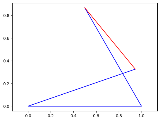
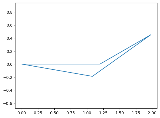
There are two solutions. Substituting in the first solution for the answer to our dependent variable (qc), we can plot it. Note that we plot the coupler in red as its position is inferred from our solution, but not explicitly solved for. If needed, this could be done in a later step

dependent = {qc:sol_n[0,0].real}
dependent

points1 = sympy.Matrix([p2.T,p1.T,o.T,p3.T]).T
points2 = sympy.Matrix([p2.T,p3.T]).T
points1_n = points1.subs({**design,**independent,**dependent})
points2_n = points2.subs({**design,**independent,**dependent})
points1_n = numpy.array(points1_n,dtype = numpy.float64)
points2_n = numpy.array(points2_n,dtype = numpy.float64)

plt.plot(*points1_n[:2],'b')
plt.plot(*points2_n[:2],'r')
plt.axis('equal')

(-0.24989304217985683,
 1.059518716294279,
 -0.04908557873865836,
 1.0307971535118254)

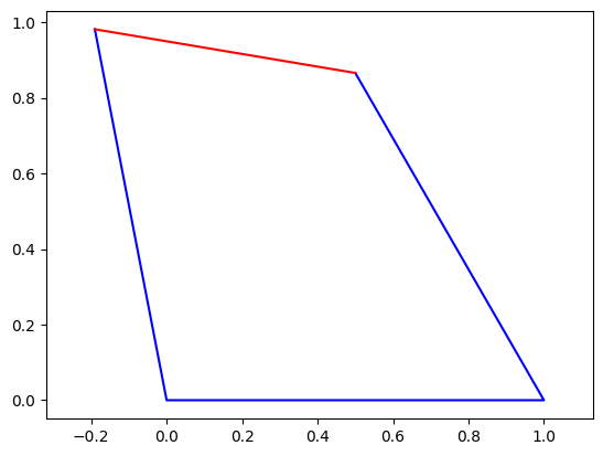
We can visualize the second solution as well:

dependent = {qc:sol_n[1,0].real}
dependent

points1 = sympy.Matrix([p2.T,p1.T,o.T,p3.T]).T
points2 = sympy.Matrix([p2.T,p3.T]).T
points1_n = points1.subs({**design,**independent,**dependent})
points2_n = points2.subs({**design,**independent,**dependent})
points1_n = numpy.array(points1_n,dtype = numpy.float64)
points2_n = numpy.array(points2_n,dtype = numpy.float64)

plt.plot(*points1_n[:2],'b')
plt.plot(*points2_n[:2],'r')
plt.axis('equal')

(-0.05, 1.05, -0.043301270189221946, 0.9093266739736607)